
Load flow and simulation of operating conditions
Load flow, sometimes known as power flow, are phrases that may be used interchangeably in power engineering. This term refers to a network solution that forecasts steady-state currents, voltages, and both real and reactive power flows across each branch and bus within the system.
 What is a Load Flow Study in Power Engineering
Load-flow studies replicate operational scenarios that cannot be feasibly encountered in the actual system due to its non-existence, temporal limitations, or the imprudence of subjecting the physical system to potentially harmful conditions.
Power systems for businesses and industries might also benefit from its use by engineers who are in charge of their electrical designs.
- What is the purpose of load flow analysis?
- The most useful load flow study applications
- How to simulate and model power system?
- Recommended courses to learn to perform load flow study
- BONUS (PDF) 🔗 Download ‘Medium voltage networks – Load flow calculation and network planning’
1. What is the purpose of load flow analysis?
The ultimate goal of the load-flow analysis is not necessarily to obtain definitive numerical performance metrics. The goal is to obtain an understanding of the system’s performance under various operating situations. And that’s it.
Power flows are a critical component of power system operation and planning and need a great attention.
The impedance of the power system network is predominantly constant due to the constant parameters of elements such as transmission and distribution lines, cables, and transformers. The impedance of the power system network is predominantly constant due to the fixed specifications of elements such as transmission and distribution lines, cables, and transformers.
Consequently, power flow computation necessitates solving a series of equations that incorporate loads of constant impedance, constant power, and occasionally constant current types.
This power flow calculation determines the electrical response of the power system to a specific set of load and supply power output.
Watch Lesson – The Concept of Power Flow Analysis
2. The most useful load flow study applications
The load flow calculation is a widespread computer approach employed in power system analysis. The planning, design, and operation of power systems necessitate computations to evaluate the steady-state performance of the system under diverse operating situations and to examine the impacts of alterations in electrical equipment configuration.
Standard outcomes from steady-state load flow analysis encompass power distribution in each branch circuit, source loading, voltage magnitude, phase angles, and other relevant parameters.
Certain equipment types, such as photovoltaic solar arrays or wind farms, necessitate a time-varying simulation, like a time domain load flow, to comprehensively analyze the electrical system’s behavior over time. The time-varying load flow solutions are executed using specialized computer programs.
Examples of load-flow study applications include determining the following:
- Component or circuit loadings
- Steady-state bus voltages
- Real and reactive power flows
- Transformer tap settings and load tap changer actions
- System real and reactive power losses and voltage drops
- Real and reactive power demand and voltage drop at utility source connection
- Generator exciter/regulator voltage set points
- Undervoltage and overvoltage conditions for buses as well as equipment terminals
- Performance under maximum, normal, minimum, and startup loading conditions
- Performance under various operating configurations (such as co-gen on or off, tie-breakers closed, etc.)
- Performance under emergency conditions (post-contingency)
- Requirement for either fixed or variable power factor improvement equipment
Watch Lesson – Load Flow Analysis Example
Load flow analysis has a great importance:
- To verify the operation of a network under various load and generation conditions
- To plan the future growth of both loads and generation
- To determine the best economical operation for existing systems
- To establish initial conditions for stability studies
- To help identify the need for additional capacitive or inductive VAR support, to maintain system voltages within acceptable limits
Nowadays, modern systems can be complicated and possess numerous pathways or branches through which power may flow. These systems constitute networks of series and parallel paths.
Electric power distribution in these networks disperses across the branches until stability is attained in accordance with Kirchhoff’s rules.
Figure 1 – Initial Load Flow Analysis
There are typically two categories of computer load flow programs: those meant for offline planning and those intended for real-time operation, actively accepting information from the actual system. The majority of load flow planning analyses employ offline software.
Online, or real-time load flows integrate data from actual networks, effectively connecting static/planning network models with those utilized by operators of the system.
Computer programs, now referred to as AI, offer integrated offline and real-time solutions for predictive analysis of “what if” scenarios. These systems can connect with current plant Supervisory Control and Data Acquisition (SCADA) systems. Integrated real-time systems can serve as both planning and design instruments, in addition to functioning as a dispatching tool for the operator.
An enhanced level of sophistication can be attained with the implementation of “optimal power flow” modeling, which incorporates limitations in the load flow solution to fulfill objectives such as minimizing fuel costs, reducing power losses, and maintaining a stable voltage profile.
A load flow calculation determines the condition of the power system based on a specified distribution of load and generation. It signifies a steady-state condition as though that condition had been maintained for a duration.
In industrial applications, certain scenarios focus on the variations in steady-state conditions over minutes to hours due to fluctuations in loading or generation; these situations can be effectively modeled using traditional load flow tools through a sequence of simulations that capture the relevant changes.
Watch Lesson – Load Flow Analysis Fundamentals
This type of study can also be conducted using a time-domain load flow program. Conversely, issues regarding system responses within the cycles-to-seconds timeframe, potentially due to short-circuits or other disruptions, must be resolved utilizing dynamic stability software.
The dynamic stability of power systems is not discussed in this technical article.
In reality, branch flows and bus voltages consistently vary slightly due to the continuous changes in loads (e.g., lights, motors, and other devices being activated or deactivated). Engineers tasked with analysis must comprehend the switching pattern and its ramifications, and may opt to disregard this when assessing the steady-state impacts on system equipment.
Load flows are fundamental for assessing new equipment installations, evaluating the efficacy of options to address current shortcomings, and fulfilling future system requirements.
The load flow model serves as the foundation for various other studies, including short-circuit, stability, motor starting, and harmonic analyses. The load flow model delivers network data and establishes an initial steady-state condition for these analyses.
Watch Lesson – Load Flow using ETAP Exercise Part #1
Watch Lesson – Load Flow using ETAP Exercise Part #2
Watch Lesson – Load Flow using ETAP Exercise Part #3
3. How to simulate and model real power system
3.1 What do we need for modeling?
Electrical systems in industrial plants can be huge. A clear visual representation of the entire system is crucial for comprehending its functionality across different operating modes. The single-line diagram of the system fulfills this function.
The single-line diagram illustrates the actual phase and neutral conductors of single-phase, two-phase, and three-phase AC systems (comprising two, three, and four wires) with a single conductor, indicating switchgear, motor control centers, loads, generators, capacitors, and interconnecting lines, cables, transformers, reactors, variable frequency drives, among others.
To study any network, we utilize electrically separate reference points, characterized by an impedance that may maintain a potential difference or by switching devices interposed between them.
The drawing format will differ based on the software utilized and user preferences; nonetheless, the single-line diagram must convey essential network and equipment information clearly and succinctly.
Figure 2 – Load flow example system single-line diagram

Understanding equipment parameters and their interrelationships is essential. Parameters may be either immediately presented on the single-line diagram or enumerated in accompanying tables, contingent upon the computer application utilized.
Figure 2 serves as a representative single-line diagram that will be utilized throughout this standard to exemplify certain elements of load-flow analyses.
Bus identifiers (usually equipment tags or numbers) are presented with the bus nominal voltages. Interconnecting lines are often represented with their impedance values and lengths specified. Devices associated with o a bus are depicted as connected to that bus. For example, generators are depicted as connected to their bus with defined equipment parameters, as demonstrated in Figure 3 and Figure 9.
Likewise, loads are depicted as connected to Bus 2A in Figure 6. Motor loads may be represented individually (e.g., MCCs) or aggregated into a single equivalent motor (“lumped“) depending on their dimensions and quantity.
Most software applications necessitate that branch elements—such as transmission lines, cables, and transformers—be interconnected between two buses.
Finally, information regarding an off-nominal turns ratio should be provided where relevant (e.g., tap settings, voltage regulator position, etc.).
Figure 3 – Single-line diagram for “Oil & Gas” substation

3.2 Overview of a power system example for industrial and commercial use
The example system designed to demonstrate the procedure of conducting a load flow analysis comprises several types of components often found in both heavy and light industrial power systems and commercial installations. Figure 2 illustrates the example system.
The following component types are present in the system:
- High-voltage switchyard: This component of the system may be owned and maintained by heavy industrial facilities.
- Switchgear for medium-voltage power distribution with several source feeders (typical of big refineries and other process-driven facilities).
- Larger cogeneration or generating facilities with a dedicated unit transformer (capacity of approximately 75 MW or more).
- Smaller generators (cogeneration, standby, and emergency).
- Double-ended secondary selective medium- and low-voltage switchgear configurations.
- Critical systems and emergency systems (such “tier 1” or “small” datacenter configurations). Uninterruptible power supply (UPS) equipment may be necessary for data backup in larger commercial or industrial locations.
- Large harmonic filters and arc furnace loads, comparable to those found in major steel production facilities. Use the right model elements from the program to replicate the harmonic load flow content and power factor correction that correspond to the features of such equipment.
- A synchronous motor having an excitation system control that may be adjusted to accommodate either voltage or power factor.
- Various induction/synchronous motor controllers can be operated by variable frequency drives (VFDs) or adjustable speed drives (ASDs).
- Photovoltaic (PV) installations, which can be connected via converters, are an example of a microgrid application that incorporates renewable energy sources.
- Wind turbine generation which can take advantage of renewable energy sources. The wind turbine system is an example of distributed generation load flow simulations.
Figure 2, which only shows a single line diagram, does not depict a real installation that incorporates all of the aforementioned components. This example was created as an educational resource for explaining load flow concepts that are typically absent in standard industrial or commercial settings.
In a real industrial facility, building loads are typically incorporated and represented as lumped loads. For the sake of simplicity, they are excluded from this example.
Figure 4 – Single-line diagram of the wind turbine

Figures 3 to 10 illustrate individual components contained within “composite networks” or components situated in other regions of the design using “remote connectors“. Composite networks are components that signify a sub-layer or hierarchical representation of items. The remote connectors are indicators that facilitate the exclusion of the connecting line between two items.
These elements do not represent a real-life element; instead, they are employed solely to facilitate the single-line drawing.
Figure 5 – Single-line diagram of the arc furnace components

Figure 6 – Single-line diagram of the ASD-driven submarine system

Figure 7 – Single-line diagram of “Substation 1” – general industrial system

Figure 8 – Single-line diagram for “Data Center”

Figure 9 – Single-line diagram of the cogeneration station

This outlines the relationships among these elements:
- The elements of the composite networks “Oil & Gas“, “Substation 1” and “Data Center” are illustrated in Figure 3, Figure 7, and Figure 8, respectively.
- The components linked via the remote connectors “Arc Furnace Feeder” and “Sub Pump Feeder” are illustrated in Figure 4 and Figure 5, respectively.
The justifications are:
- The standard symbol lacks the complexity necessary to visually communicate the technical specifics of the component.
- IEEE standards may not align with current technology, or the symbols may be specific to the software.
- Compound elements, such as lumped loads and photovoltaic arrays, necessitate many symbols for their representation. Software products may employ alternative “compound symbols” to facilitate the drawing process.
The reasons listed above explain why the majority of software products may not employ a uniform set of symbols. Table 1 presents details regarding the symbols utilized in the power system analysis program illustrated in this particular example.
Table 1 – Element symbols used for computer software example

Figure 10 – Single-line diagram for the unit generation plant

4. Recommended courses
4.1 Power System Analysis, Modelling, Load Flow and Fault Studies for True Engineers
In this class, you will learn everything there is to know about power system analysis, beginning with the fundamentals of single phase and three phase electric systems, moving on to the designing and modeling of various power system components like generators, transformers, and transmission lines, and concluding with a complete power system study that includes load flow studies and an analysis of power system faults.
Therefore, you can consider this class to be your comprehensive reference to one of the most important subfields of power engineering: an examination or analysis of the power system.
The course consists of 15 chapters, 121 lectures and 21h 41m total length.

4.2 Power System Analysis Course: The Essentials of Load Flow and Short Circuits
This course is dedicated to one of the main areas of electrical engineering: power system analysis. Power system analysis is the core of power engineering and its understanding is therefore essential for a career in this field. In this course, you will learn about power flow (load flow) analysis and short circuit analysis and their use in power systems.
The course consists of 37 lectures in 5h 48m total length., and it’s divided into the following sections:
- Power flow (load flow) analysis
- Short circuit analysis of balanced and unbalanced faults
- Advanced concepts in Power Engineering
- Calculate the bus admittance matrix of a power system
- Symmetrical Components

4.3 ETAP Power System Design and Analysis Course: Learn To Resolve Power System Issues
This course provides a knowledge in power system modeling and analysis by utilizing the ETAP program and its features. This will enable you to effectively design and resolve different actual power system issues.
You will acquire the knowledge and skills to model and evaluate the steady-state and dynamic power system, and to perform various analysis such as arc-flash analysis, transient stability, motor accelerating analysis, short-circuit analysis, harmonics analysis, protection example, earthing analysis and an example of renewable energy sources.
The course consists of a total of 34 lessons and has a duration of 5 hours and 29 minutes.
The course will begin with the ETAP software overview, basics of single-line diagram creation, data entry, and quickly expands the users’ knowledge to include methods to automatically perform multiple ‘what if’ studies using multiple scenarios.

5. BONUS (PDF): Medium voltage networks – Load flow calculation and network planning
Download: Medium voltage networks – Load flow calculation and network planning (for premium members only):
Reference: IEEEStd3002.2™-2018
Related electrical guides & articles


Edvard Csanyi
Hi, I'm an electrical engineer, programmer and founder of EEP - Electrical Engineering Portal. I worked twelve years at Schneider Electric in the position of technical support for low- and medium-voltage projects and the design of busbar trunking systems.I'm highly specialized in the design of LV/MV switchgear and low-voltage, high-power busbar trunking (<6300A) in substations, commercial buildings and industry facilities. I'm also a professional in AutoCAD programming.
Profile: Edvard Csanyi

kedves Csányi Úr!
Gratulálok az oldalhoz és az üzleti sikerhez!
Színvonalas magas igényű.
Véghely Tamás okl. vill. mérnök, gyenge áram
napelem szakértő
+3630 9967675
I am electrical engineering ( industrial control )